OFFSET Function. Get a cell by specifying the distance from the reference cell, height and width.(Microsoft Excel)
The OFFSET function is a cell specification function.
The argument is the number of rows and columns away from the base cell, and the width and height of the cell.
It can return the value of a single cell or a range of cells.
How it works
=OFFSET(Reference,Rows,Cols,Height,Width)
| Name | Omission | Explanation |
|---|---|---|
| Reference | Required argument. Specify a reference cell range. | |
| Rows | Required argument. Specifies the distance (number of lines) from the "reference". | |
| Cols | Required argument. Specifies the distance (number of columns) from the "reference". | |
| Height | Same number of rows as in "Reference. | |
| Width | Same number of rows as in "Reference. |
If the height and width are set to 1, the cell is a single cell and the value can be displayed as is.
If the height or width is set to 2 or greater, it becomes a cell range and If not incorporated into another function, it will be a Spill.
Versions that do not support Spill will result in a #VALUE
Demonstrate
The reference cell has a yellow background.
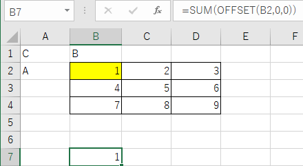
Example of getting single cell.
If both the number of rows and the number of columns are set to 0, the result will be the reference cell, and in the example, 1 is displayed.
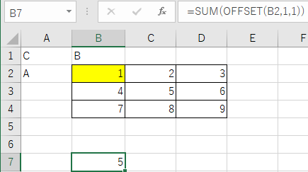
Setting both the number of rows and the number of columns to 1 specifies that the cell is one column to the right and one row below the reference cell. In this example, 5 is displayed.
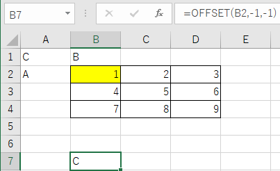
If a negative value is specified, the designation is the upper left corner, and in this example, C is displayed.
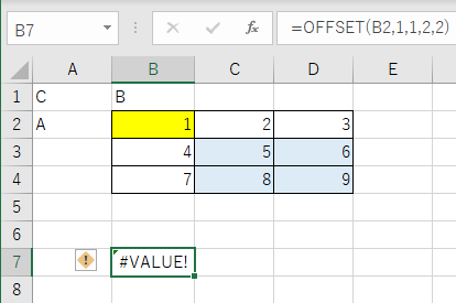
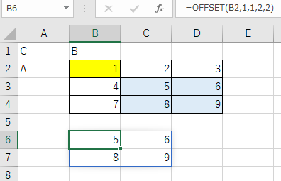
Example of getting cell range.
Moves 1 right and 1 down from the reference cell, specifying a height of 2 and a width of 2. (range with blue background color)
In this case, the display will show a #VALUE because the cell is not alone.
(In the case of a version that does not support spills)
If the spill is a valid version, it will be a Spill.
The results of the OFFSET function can be incorporated into other functions.
If we incorporate the previous example as a range in the SUM function
28, which is the sum of the range with blue background color, will be displayed.