

The SUMIFS function displays the sum of cells that satisfy multiple conditions.
It is a higher version of the SUMIF function (with one condition and one condition range).
How it works
=SUMIFS(Sum_range,Criteria_range1,Criteria1 ... omit ... Criteria_range127,Criteria127)
| Name | Omission | Description |
|---|---|---|
| Sum_range | Required fields | Specifies a range of cells to be summed. Non-numeric cells within the total range are excluded. |
| Criteria_range1 - 127 | Only 1 is required. | Specifies a range of cells to be evaluated for the condition. |
| Criteria1 - 127 | Only 1 is required. | Specify the conditions to be included in the total. |
Demonstrate
For example, it can be used to total sales in a specific category of products and only those sales that are eligible for discounts.
It can also be used in cases where a comparison of large and small items is required, such as totaling all sales that are on sale and above a certain unit price.
The following is an example of a SUMIF function that refers to the table below.

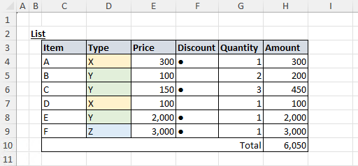
Example of summing data matching a specific string
This is an example of searching and summing the amounts in the source table that match the type in column C and are subject to discount.
Column D is the total result using the SUMIFS function.
=SUMIFS(Sheet1!$E$4:$E$9,Sheet1!$D$4:$D$9,Sheet2!C4,Sheet1!$F$4:$F$9,"●")

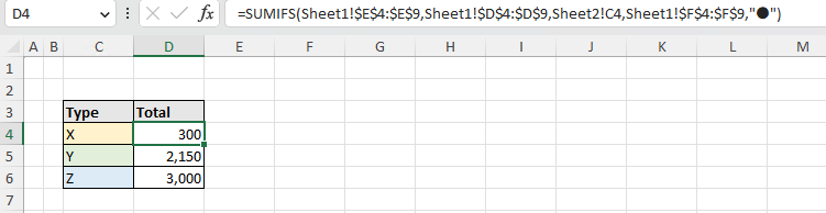
Criteria_range1~2 and Sum_range are specified by absolute cell reference so that they are fixed even if copied, since the referenced list remains unchanged even if the position is changed by copying.
In this case, the reference is an exact match, but it is also possible to use wildcards to specify a partial match.
Example of totaling with a numerical threshold
This is an example of totaling the sum of amounts that are above a specific unit price and are subject to a discount.
Column D is the total result using the SUMIFS function.
=SUMIFS(Sheet1!$E$4:$E$9,Sheet1!$F$4:$F$9,"●",Sheet1!$E$4:$E$9,">="&Sheet4!B3)

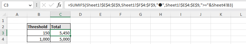
It is possible to set conditions such as above or below a specific number by specifying a comparison operator in the condition.
In the example here, the first line shows the total of all discount items with a unit price of 150 yen or more, and the second line shows the total of all sale items with a unit price of 1,000 yen or more.
Note that comparison operators must be enclosed in "(double-cotation marks)" and treated as character strings.
The & (ampersand) is the string concatenation operator.
The result of ">="&C21" is ">=150".
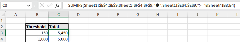
Spill
If a cell range is specified for the "Criteria", it will be Spill.
=SUMIFS(Sheet1!$E$4:$E$9,Sheet1!$F$4:$F$9,"●",Sheet1!$E$4:$E$9,">="&Sheet4!B3:B4)

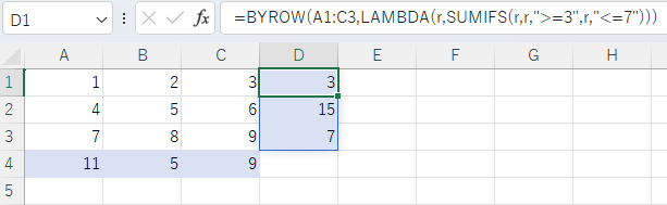
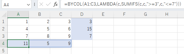
Also, Spill when using the BYROW or BYCOL function.
=BYROW(A1:C3,LAMBDA(r,SUMIFS(r,r,">=3",r,"<=7")))

=BYCOL(A1:C3,LAMBDA(c,SUMIFS(c,c,">=3",c,"<=7")))

---