

Here is a formula that performs a cross tabulation in Spill.
This formula automatically reflects the increased data when the source data for cross tabulation increases, without the need to edit the cross tabulation sheet.
Functionally, it is similar to what can be done with a pivot table.
If that is sufficient, there is no need to use Spill.
The advantage of this method over pivot tables is that it does not require manual updating of data.
Therefore, when performing multiple cross tabulations from the same data
Spill is more advantageous because there is no need to update the data.
Note that this method may not be available for older versions of Excel because it uses the latest functions.
Cross tabulation samples.

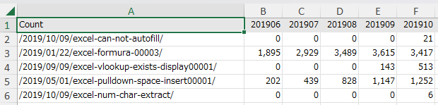

Formula
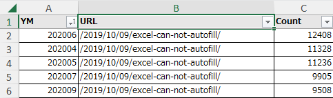
The vertical direction of the cross tabulation is the URL. Create its header row in column A.
Set up the formula below in cell A2 using the LET, SORT, UNIQUE, and FILETER functions.
=LET(
  URL_cell_range,Data!B:B,
  SORT(UNIQUE(
    FILTER(URL_cell_range,(URL_cell_range<>"")*(URL_cell_range<>"URL"))
  ))
)

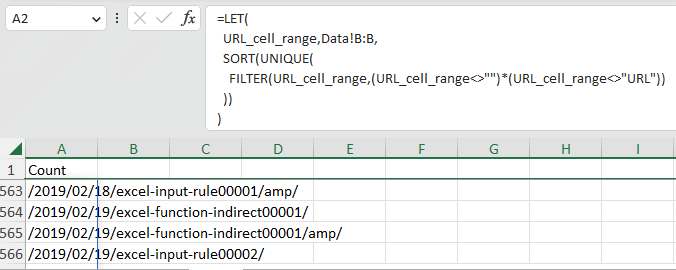
The FILTER function extracts rows from a range of cells that satisfy certain conditions.
The first argument specifies the cell range and the second argument specifies the extraction conditions.
The first half of the condition is to exclude blank cells, and the second half is to exclude header rows.
The "*" is a logical conjunction.
(URL range<>"")*(URL range<>"URL")
This will retrieve rows that are neither blank nor headers.
The UNIQUE function excludes duplicates in a cell range.
The SORT function reorders the specified range. (Not necessary if there is no need to reorder.)
This completes the vertical header row.
Next is the horizontal year and month. Create its header row on the first line.
Enter the following formulas in cell B1 using the TRANSPOSE, SORT, UNIQUE, and FILTER functions.
=LET(
  YM_cell_range,Data!A:A,
  TRANSPOSE(SORT(UNIQUE(
  FILTER(YM_cell_range,(YM_cell_range<>"")*(YM_cell_range<>"YM"))
  )))
)

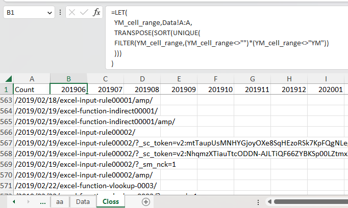
It's almost identical to the formula in the URL, except for the cell range and the condition.
The TRANSPOSE function is used at the end to switch from vertical to horizontal direction.
This completes the horizontal header row.
Finally, we create the formula for the aggregate data: in cell B2, we set the following formula using the SUMIFS function.
=SUMIFS(
  Data!C:C,
  Data!A:A,B1#,
  Data!B:B,A2#
)
B1# and A1# are range specifications for the entire spill, not just individual cells.

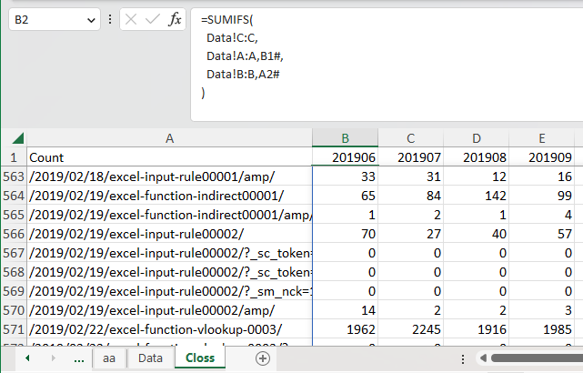
The cross tabulation table is now complete with formulas for only 3 cells, A2, B1, and B2.
If new years, months, or URLs are added to the data sheet
The cross tabulation table will be automatically expanded. (However, if manual tabulation is used, it will not be automatic.)
In this case, the SUMIFS function is used to total the data, but the AVERAGEIFS, MAXIFS, MINIFS, and COUNTIFS functions can be used as well.
GROUPBY or PIVOTBY function
In some cases, the GROUPBY function or PIVOTBY function, which were added in the September 2024 update, can be used to resolve the update issue without using a pivot table.
Use the GROUPBY function if there is one aggregate axis, and the PIVOTBY function if there are two.
In cases where the GROUPBY function or PIVOTBY function can be used, this may be more efficient.
---