

The LET function is a new function added in September 2020 to make formulas easier to read and improve calculation speed.
For those who have experience with some programming language or macros, it is easier to understand if you think of it as being able to use variables in formulas.
How it works
=LET(Name1, Value1, Name2, Value2, ... , Name126, Value126, Formula )
| Name | Omission | Explanation |
|---|---|---|
| Name1 to 126 | Required argument. Must begin with a non-numeric value. At least one name and value set must be specified. After 2, up to 126 can be specified. | |
| Value1 to 126 | Required argument. Specify the content corresponding to the name. It can be a number, a string, or an equation. | |
| Formula | Required argument. This is the last argument, the odd-numbered argument. This will be a formula that uses the names defined so far. |
Demonstrate
Basic.
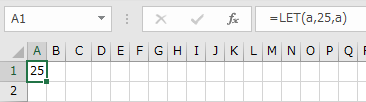
=LET(a,25,a)
| Argument | Value |
|---|---|
| Name1 | a |
| Value1 | 25 |
| Formula | a |
In the last formula, the name a is treated as 25, without the " since a is not a string.
(Same as Name Manager.)

Text for value.
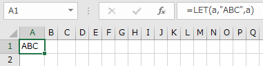
A string can be specified by enclosing the value in ".
=LET(a,"ABC",a)
| Argument | Value |
|---|---|
| Name1 | a |
| Value1 | "ABC" |
| Formula | a |

Multiple names define.
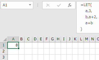
Here is an example of defining multiple names.
If the formula is long, it is easier to read if a new line is inserted in the cell for each set of names and values.
Also, for values 2 through 126, names already defined further to the left can be used.
=LET(
  a,3,
  b,a+2,
  a+b
)
| 引数 | 設定値 |
|---|---|
| Name1 | a |
| Value1 | 3 |
| Name2 | b |
| Value2 | a+2 |
| Formula | a+b |
a=3, b=5. 3+5 yields 8.

important point
The ET function is a useful but new function that is not well known and is quite different in nature from previous Excel formulas.
Therefore, it is better to explain the LET function if there is a possibility that others will see the formulas.
Situation in which the LET function is valid.
It is necessary to determine if it is appropriate, because if used unintentionally, the formulas will be difficult to understand.
Specify the same formula multiple times. Redundant formulas.
For example, in the formula below, there are two identical VLOOKUP functions.
=IF(VLOOKUP(C2,B6:C8,2,FALSE)="","",VLOOKUP(C2,B6:C8,2,FALSE))
It can be improved with the formula below.
=LET(vl,VLOOKUP(C2,B6:C8,2,FALSE),IF(vl="","",vl))
The ability to combine identical formulas under one name eliminates the possibility of changing only one function and forgetting to change other identical parts of the function.
Even simple cell references can be effective if there are a large number of references to the same location.
This is also effective in cases where intermediate cells are created and formulas are omitted.
It also improves calculation speed as the function is executed only once to store the calculation results.
In the previous example, two VLOOKUP function executions can be done once.
The improvement in calculation speed is particularly effective when using a large number of functions that tend to be slow, such as the FIND, XLOOKUP, and VLOOKUP functions.
Simplify complex mathematical formulas.
It is also useful to simplify complicated mathematical expressions by naming them in fixed chunks.
The following example works in conjunction with deduplication.
=MID(B3,FIND(C3,B3)+LEN(C3),FIND(D3,B3)-FIND(C3,B3)-LEN(C3))

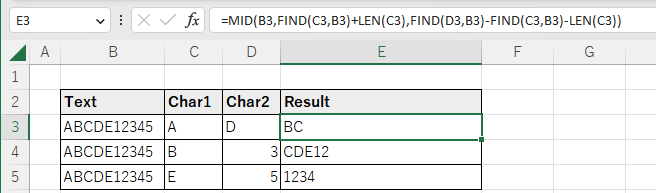
The main idea is to use the MID function to cut out the string of characters between the characters in column C and the characters in column D. However, the FIND and LEN functions to determine the position of the cutout are intricate.
There are also duplicate formulas that are colored with the background color.
If we first deduplicate only, we get the following formula.
=LET(
  Character1Position,FIND(C3,B3),
  Character1Length,LEN(C3),
  MID(B3,Character1Position+Character1Length,FIND(D3,B3)-Character1Position-Character1Length)
)
Naming and clarifying the meaningful parts of the equation leads to the following formula.
=LET(
  Character1Position,FIND(C3,B3),
  Character1Length,LEN(C3),
  StartPosition,Character1Position+Character1Length,
  ExtractLength,FIND(D3,B3)-Character1Position-Character1Length,
  MID(B3,StartPosition,ExtractLength)
)
This clarifies the structure of the MID function formula.
---