

When there are multiple results that match the search criteria of the VLOOKUP function, the first matching result is retrieved.
Here we will show you how to retrieve the last matching result instead of the first.
Formula
The sample below illustrates this.
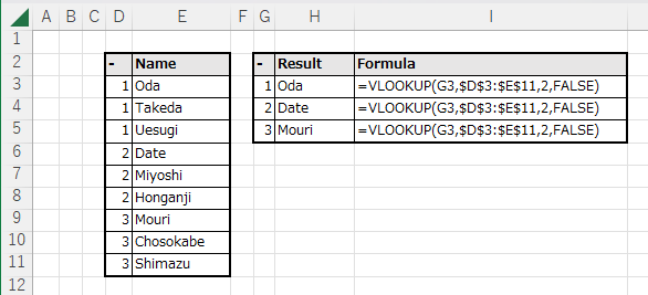
Columns D and E are the tables to be searched and column H is the column for the VLOOKUP function.
In the normal use of the VLOOKUP function, if 1 is specified for the search value
the first match will be Oda, 2 will be Date, and 3 will be Mouri.

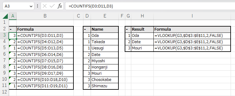
Add a column for the COUNTIFS function and copy the formula. In the sample, this is column A.
=COUNTIFS(D3:D11,D3)

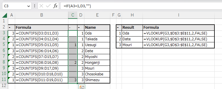
Next, add the columns for the IF function. In the sample, this is column C.
This is a formula to ensure that the value to be searched is displayed in the cell only if column A is 1.
=IF(A3=1,D3,"")

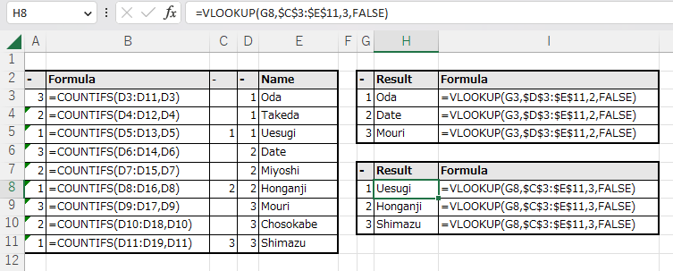
Create a VLOOKUP function with this IF function column as the search target and you are done. In the sample, the cells are H8 to H11.

For the XLOOKUP function.
In the XLOOKUP function, the match_mode argument can be used to specify whether to retrieve from the beginning or from the end.
This is very convenient because it can be achieved using only the XLOOKUP function without using the IF and COUNTIFS functions.
---