

The VLOOKUP function is a versatile function in Excel for retrieving cell values and is a guidepost for intermediate Excel users. However, the latest Excel version introduces a more powerful XLOOKUP function.
Features of the XLOOKUP function:
- Combines the functionality of the VLOOKUP and HLOOKUP functions
- Eliminates many limitations of the VLOOKUP function
- Allows more flexible and efficient searching
If you are using a newer version of Excel, you may want to consider moving to the XLOOKUP function. This will make data analysis and table manipulation easier and more efficient.
However, if compatibility with older versions of Excel or file sharing with other users needs to be considered, choose the appropriate function for your situation.
By taking advantage of the benefits of the XLOOKUP function while also maintaining knowledge of the VLOOKUP function as needed, you will develop flexible Excel skills that can be used in a variety of situations.
How it works
=VLOOKUP (lookup_value, table_array, col_index_num, range_lookup)
| Name | Omission | Explanation |
|---|---|---|
| lookup_value | Required argument. | Specify the value (search key) to be searched. |
| table_array | Required argument. | Cell range to search. The column to look for the search value must be the leftmost column, and include the column from which to retrieve the results. |
| col_index_num | Required argument. | Specifies the column in which to display the search results."Sequential number of table_array with the leftmost column as 1. |
| range_lookup | TRUE | FALSE: Obtain an exact match. TRUE: Get the largest match under the search key. |
Demonstrate
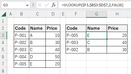
The most common usage is to match the ledger with a code, etc., to retrieve and display information such as names and prices.
This can eliminate posting errors.
In the example below, the code in column F is retrieved from column B, and the corresponding product name and price are automatically displayed.
Argument 1: lookup_value
In the example, we specify the Code in column F.
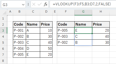
Given the use of auto-fill and copy & paste
it is safer to fix the specification of column F with an absolute cell reference.

Comparison operators are not allowed here. Specify the string you want to match.
Forward, partial, and backward matches are also possible, but since the VLOOKUP function itself searches a single cell, it is not suitable for displaying multiple search results.
Use a combination of other functions or use the FILTER function.
Argument 2: table_array
Note that the column to look for the search value must always be the leftmost column. If you want to search for a column other than the leftmost column, you must be creative.
If you want to search for Code as in the example, the leftmost column of the range must be Code.
The XLOOKUP function improves on this point by allowing the search to be performed even if the left-most column is not the left-most column.
If you are copying formulas to multiple cells, it is safer to fix the formulas to named ranges or columns by absolute cell reference only, rather than by cell specification.
Argument 3: col_index_num
The items to be retrieved as a result.
In this example, 1 displays the code, 2 the product name, and 3 the price.
In the XLOOKUP function, it is a cell range, not a number.
Absolute cell reference are also possible, making it more convenient.
In addition, images can now be used in the search results.
Argument 4: range_lookup
In most cases, FALSE is specified for an exact match.
If TRUE is specified, the E of P-005 will be retrieved when P-006, which does not exist, is specified.
If FALSE is specified, there are no results for P-006.
When omitted, the result is TRUE, which is inconvenient for beginners. However, in the XLOOKUP function, FALSE is used as the omitted value, which is a great improvement.
If there is no match.
If the search result does not exist, it will result in a #N/A error, which will adversely affect other expressions.
If it is only a display problem, there is no serious impact even if it is left as it is.
However, it is not desirable to have the error remain in the documentation, so we recommend that it be addressed.
In the XLOOKUP function, this can be handled with an argument.
Spill
If you specify the argument "lookup_value" the cell range, it will be Spil.

---