

In the VLOOKUP function, the column to be searched must be the leftmost column.

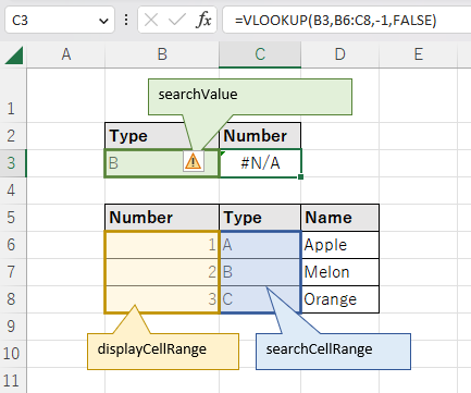
In this example, we specify Type in cell B3 and
I want to get the corresponding Number in cell C3.
In the table B6 to D8, Number is to the left of Type, so it is impossible to use the VLOOKUP function normally.
Many tables basically have the number or code at the left end and the name or name to the right of the number or code.
Four ways.
- Use the XLOOKUP function.
- Move the search column to the left.
- Create a column with only cell references on the left.
- Use the INDEX and MATCH functions.
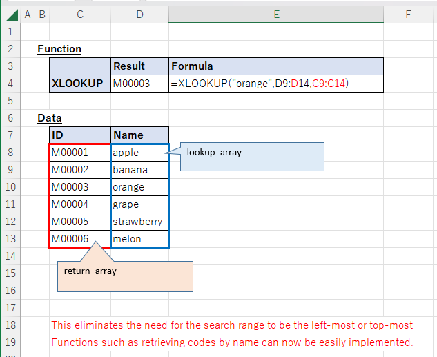
Use the XLOOKUP function.
In January 2020, a very useful higher-level version of the XLOOKUP function was added.
This function changes the way to specify the search range and can be used even if the search range is not on the left side.

Move the search column to the left.
Change the table structure and move the column to be searched to the far left.
If this is a temporary use, creating disposable sheets can be useful.
If changing the table structure is not a problem, this is the easiest and most fundamental solution.
Create a column with only cell references on the left.
It is also useful to create a column on the left end that is just a cell reference to the column to be searched.
This also changes the structure of the table, but requires only a simple formula with cell references.
Also, if the left-most column is not used for any other purpose, it can be made invisible by hiding the column. If the leftmost column is not used for any other purpose, it can be hidden from view.
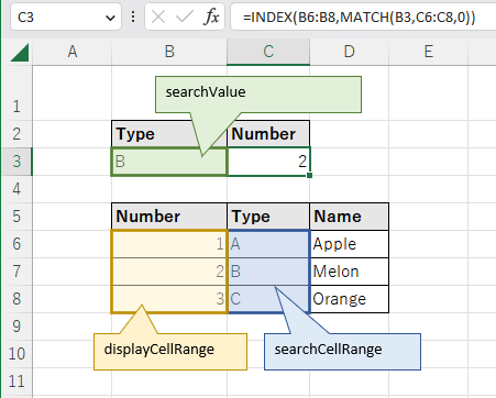
Use the INDEX and MATCH functions.
If you do not want to manipulate the table structure, use the INDEX and MATCH functions.
=INDEX(displayCellRange,MATCH(searchValue,searchCellRange,0))

---