

Pivot tables do not support median values.
This article shows how to achieve this using only formulas, without add-ins or macros.

GROUPBY or PIVOTBY function
The GROUPBY function and PIVOTBY function, which were added in the September 2024 update, work in the same way as pivot tables, but the median can be used as a method of aggregation.
Use the GROUPBY function when there is one axis of aggregation, and the PIVOTBY function when there are two axes.
If you are in an environment where you can use the GROUPBY function and PIVOTBY function, and you don't need to change the axis of aggregation frequently, we recommend using these functions instead of pivot tables.
Procedure
Pivot tables are often when you want to aggregate on one or more axes, like years and months.
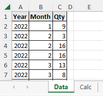
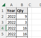
In the sheet below, I will show you an example of using the year in column A and the month in column B as the axes.

Create an item row at the top of the tabulation sheet (Item rows are not required)

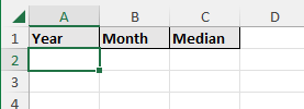
Set the UNIQUE function in cell A2.
The argument is the column of the axis year and month, column A:B of the Data sheet.
=UNIQUE(Data!A:B)

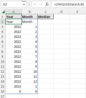
Since the top of the UNIQUE function result is the item row and the bottom is a row with only 0s, the DROP function is stacked to delete.
If there are no item rows on the Data sheet, only the -1 DROP function is needed to delete the tail.
=DROP(DROP(UNIQUE(Data!A:B),1),-1)

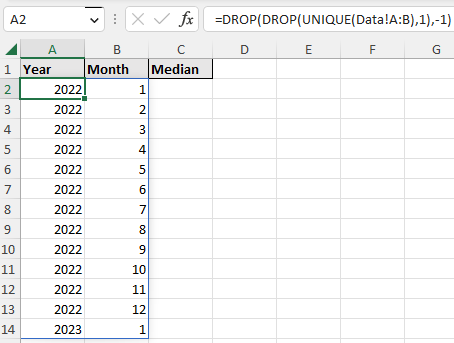
The formula is only in cell A2, but it is a spill and will automatically reflect any new values added to the Data sheet, such as February 2023.
You can use for SUMIFS and AVERAGEIFS, but they do not exist in MEDIAN.
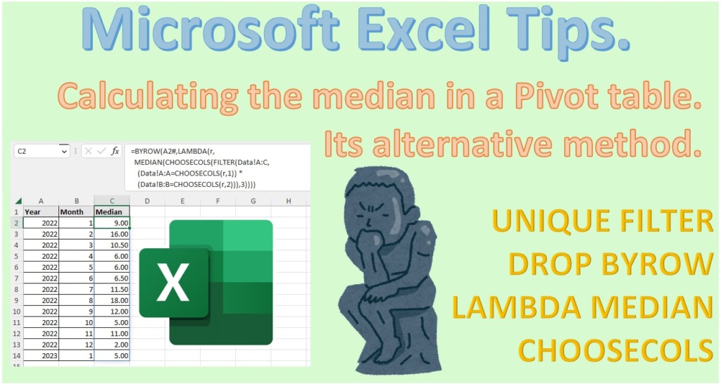
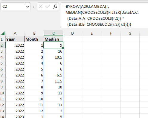
Instead, set the following formulas in cell C2 using the following BYROW, LAMBDA, MEDIAN, CHOOSECOLS, and FILTER functions.
=BYROW(A2#,LAMBDA(r,
  MEDIAN(CHOOSECOLS(FILTER(Data!A:C,
    (Data!A:A=CHOOSECOLS(r,1)) *
    (Data!B:B=CHOOSECOLS(r,2)))
  ,3))))
This formula calculates the median value for each year, and the Data sheet will be in a state to automatically reflect any new values added, such as February 2023.

Modification example
Calculate other than median
Any other aggregate function will result in a non-median value, so there is no advantage to an aggregate function that has IFS or that does not exist in a pivot table. SNGL for mode mode.
=BYROW(A2#,LAMBDA(r,
  MODE.SNGL(CHOOSECOLS(FILTER(Data!A:C,
    (Data!A:A=CHOOSECOLS(r,1)) *
    (Data!B:B=CHOOSECOLS(r,2)))
  ,3))))
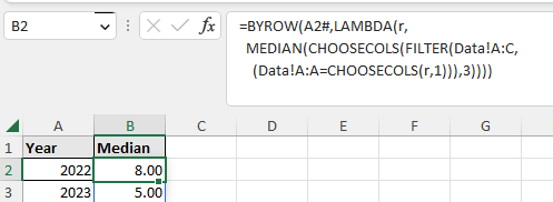
One axis
The number of formulas is reduced because there are fewer columns of data.
=BYROW(A2#,LAMBDA(r,
  MEDIAN(CHOOSECOLS(FILTER(Data!A:C,
    (Data!A:A=CHOOSECOLS(r,1)))
  ,3))))
Below is a formula with two axes. (The changed parts are in red)
=BYROW(A2#,LAMBDA(r,
  MEDIAN(CHOOSECOLS(FILTER(Data!A:C,
    (Data!A:A=CHOOSECOLS(r,1)) *
    (Data!B:B=CHOOSECOLS(r,2)))
  ,3))))

If the Data sheet has only a year column, the formula changes.

=BYROW(A2#,LAMBDA(r,
  MEDIAN(CHOOSECOLS(FILTER(Data!A:B,
    (Data!A:A=CHOOSECOLS(r,1)))
  ,2))))
The last number is the column that aggregates the median value within the cell range specified by the FILTER function. (The leftmost is a sequential number of 1's)
Three axes.
More columns are added to the Data sheet.

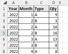
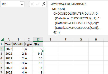
The formula is below. The last number has changed from 3 to 4, which specifies how many columns in the Data sheet are to be counted. The number of items has been increased by one because the type column has been increased and the number of items has been moved to the right by one.
=BYROW(A2#,LAMBDA(r,
  MEDIAN(
    CHOOSECOLS(FILTER(Data!A:D,
      (Data!A:A=CHOOSECOLS(r,1))*
      (Data!B:B=CHOOSECOLS(r,2))*
      (Data!C:C=CHOOSECOLS(r,3))),
    4))))

---