INDEX Function. Retrieves values by specifying range of cells, number of rows, and number of columns.(Microsoft Excel)
The INDEX function is a function that retrieves the value of a cell by specifying the cell range, row number, and column number.
It is rarely used by itself, but in combination with other functions.
How it works
=INDEX(array, row_num, column_num,area_num)
| Name | Omission | Explanation |
|---|---|---|
| array/reference | Required argument. | |
| row_num | 0 | Required field if there is no column_num. The number of rows to take out of the array/reference. The top row is 1. |
| column_num | 0 | Required field if there is no row_num. Specifies numerically how many rows to take out of the array/reference. The leftmost column is 1. |
| area_num | If multiple cell ranges are specified in an array/reference, specify by number which cell range is used. The first cell range is 1. |
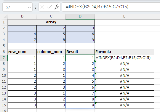
Demonstrate
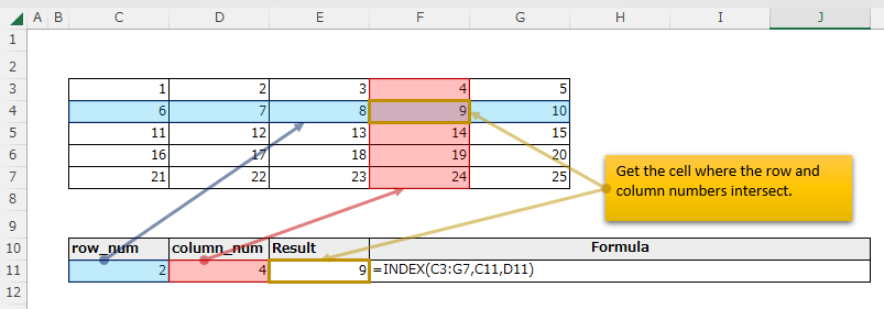
Here is an example of searching a blue cell range with the INDEX function.
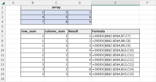
The INDEX function retrieves the cell where the row and column numbers intersect.
Omitting the column_num or setting it to 0 results in a Spill that retrieves the entire row.
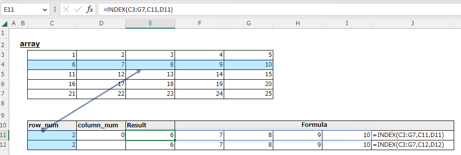
If the row_num is omitted or set to 0, it will be a spill that retrieves all of that column.
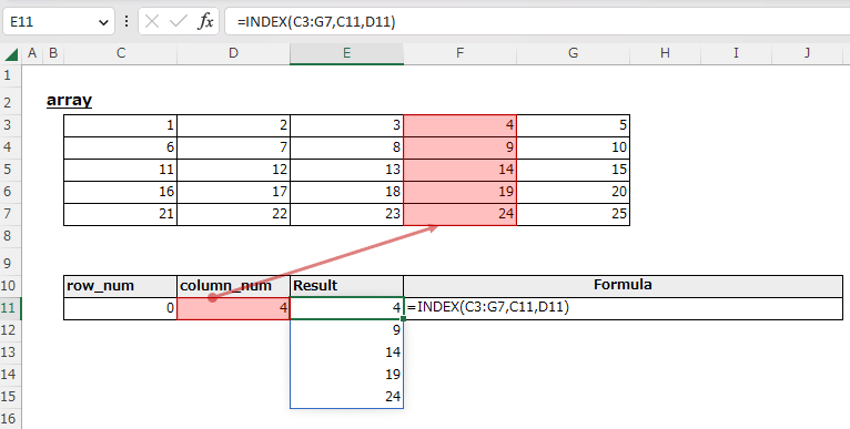
Specifying more than the range will result in a #REF! error.
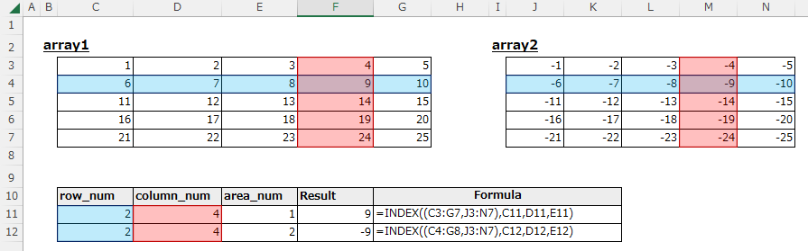
Argument 4: Use of area_num
The area number in argument 4 is an argument that specifies which range to use when multiple ranges are specified by the reference operator.
Specify (C3:G7,J3:N7) for argument 1. () is required.
Then, specify the area number as argument 4.
If 1 is specified for the area number, the search starts from C3:G7, and if 2 is specified, the search starts from J3:N7.
In practical use, it is assumed that the IF function or SWICTH function is used to select an area under certain conditions.
Spill
If you specify the argument "row_num" or "col_num" the cell range, it will be Spil.
---