FILTER function. Get all rows matching the condition.(Microsoft Excel)
The FILTER function is a related function of Spill that was implemented in 2019 to retrieve data that matches certain criteria.
How it works
=FILTER(array,include,if_empty)
| Name | Omission | Explanation |
|---|---|---|
| array | Required argument. Cell range to filter. | |
| include | Required argument. Search criteria. | |
| if_empty | #CALC | Result for 0 case. |
Demonstrate
Basic.
Arrays and Includes.
The first argument specifies the range of the source data, and the second argument specifies the search condition.
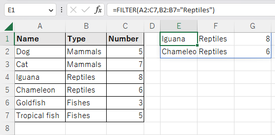
In the example below, we extract rows whose Type is Reptiles.
=FILTER(A2:C7,B2:B7="Reptiles")
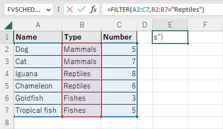
If you enter the FILTER function in one cell, it will automatically expand to match the number of results of the condition.
Cells other than the original cell where the function was first entered are Ghost and cannot be edited.
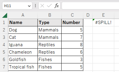
However, if there is any value in the auto-expand destination cell, it will result in a #SPILL.
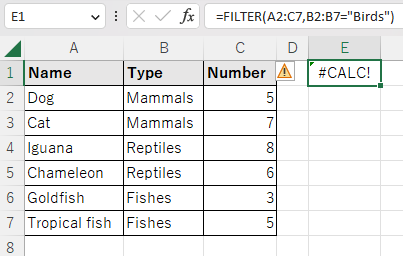
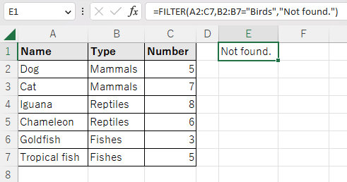
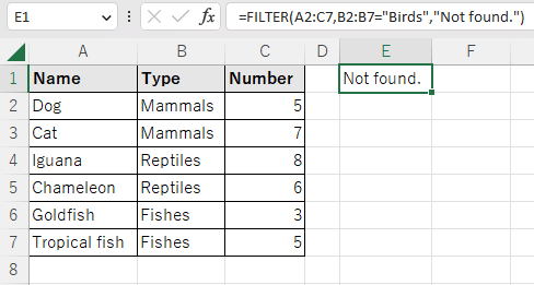
If empty.
The third argument specifies the result if not found.If not specified, #CALC!
If specified, the result is the case where the specified value is not found.
If specified, the result is the case where the specified value is not found.
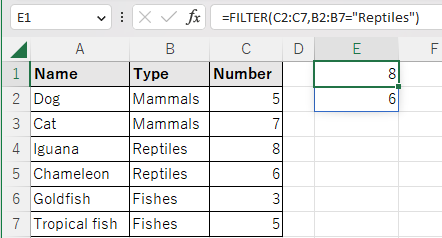
If you want to get only a specific column.
The range of argument 2 need not be included in argument 1.
If you specify only the columns you want to display in argument 1, you can retrieve only those columns.
=FILTER(C2:C7,B2:B7="Reptiles")
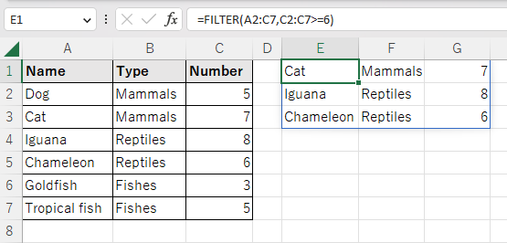
Large and small conditions.
In the example below, data with Number greater than 6 are extracted.
=FILTER(A2:C7,C2:C7>=6)
Multiple conditions.
| - | operator |
|---|---|
| AND | * |
| OR | + |
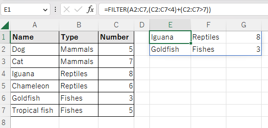
Disjunction
The following is an example of using + to extract data where "Number" is less than 4 or greater than 7.
=FILTER(A2:C7,(C2:C7<4)+(C2:C7>7))
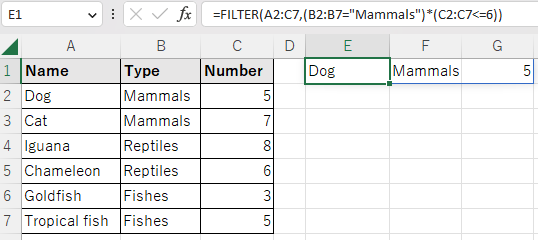
logical conjunction
The following is an example of using * to extract data that is Mammals and less than or equal to 6.
=FILTER(A2:C7,(B2:B7="Mammals")*(C2:C7<=6))
Substring Match
Wildcards are not available, but partial match searches can be performed in conjunction with other functions.
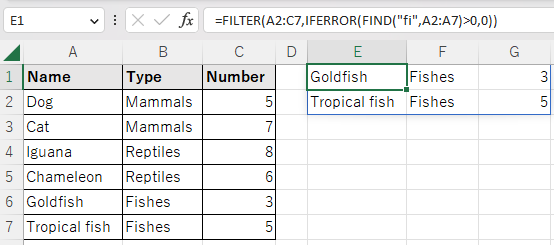
FIND and IFERROR functions. Substring Match
The FIND and IFERROR functions can be used to perform partial match searches.
=FILTER(A2:C7,IFERROR(FIND("fi",A2:A7)>0,0))
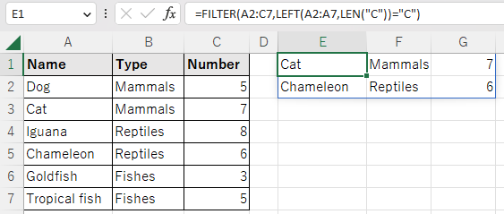
LEFT and Len Functions. Forward Match.
Forward matching conditions are possible with the LEFT and LEN functions.
=FILTER(A2:C7,LEFT(A2:A7,LEN("C"))="C")
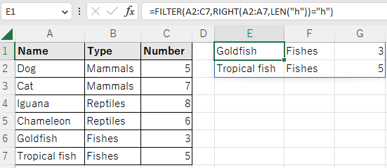
RIGHT and Len functions. Backward matching.
Backward matching is possible with the RIGHT and LEN functions.
=FILTER(A2:C7,RIGHT(A2:A7,LEN("h"))="h")
Date/time conditions. Date & Time functions.
You could make the serial value a condition, but
However, it is more difficult to enter, and the formulas are more difficult to understand.
Therefore, you should use the date entered in the cell as the condition or use the Date & Time function together.
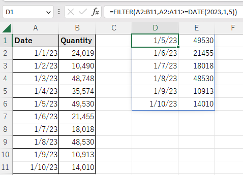
For example, the DATE function can be used to compare dates without using serial values.
=FILTER(A2:B11,A2:A11>=DATE(2023,1,5))
Use results for other functions
SORT and SORTBY functions.
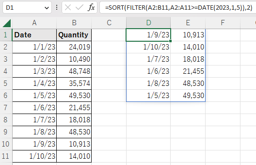
Since the result of the FILTER function is a range of cells, it can be passed to other functions that take a range of cells as an argument.
For example, the results of a FILTER function can be sorted by a SORT or SORTBY function.
=SORT(FILTER(A2:B11,A2:A11>=DATE(2023,1,5)),2)
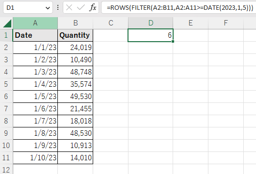
Get the number of results with the ROWS function.
Specifying the result of the FILTER function as the argument of the ROWS function results in the number of cases matching the condition.
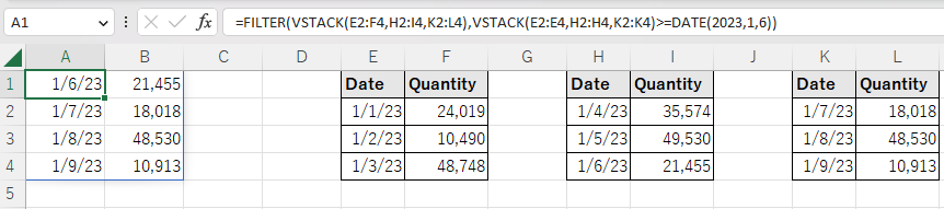
Multiple cell ranges.
Multiple ranges can be targeted with the VSTACK and HSTACK functions.
---